Table of Contents Introduction: The Collapse of Flat-Vector RAG The RAG Maturity Model: From Flat Chunks to Layered Memory Tiers Hybrid Retrieval Mechanics: Mer…
Introduction: The Collapse of Flat-Vector RAG
In 2023, building a Retrieval-Augmented Generation (RAG) system was simple: take a collection of PDF files, cut them into arbitrary 512-token chunks with a 10% overlap, generate vector embeddings using a public model API, store them in a vector database, and perform a cosine similarity lookup against a user's prompt.
This naive approach, which we can call RAG 1.0, worked well for basic query-response demos. However, as organizations attempted to deploy these systems into production for complex enterprise tasks, the architecture began to break down.
In production environments, naive vector retrieval suffers from significant limitations:
- Loss of Structural Context: Dissecting a document into disjointed chunks strips away hierarchical relationships. An agent cannot easily determine if a chunk belongs to a specific subsection of a safety protocol, a warning paragraph in an appendix, or an unrelated contract.
- Domain-Specific Mismatch: Dense vector models are trained on general web text. They struggle to match specialized queries—such as looking up product codes like
X-402-V2or distinct internal tracking codes—because these specific terms lack semantic neighbors in public embedding spaces. - Multi-Hop Failure Modes: Vector search retrieves individual chunks based on overall semantic similarity. If a user asks a complex question that requires combining information from multiple different sources—such as "which component in Project Alpha was updated after the May security audit?"—a simple vector similarity query will fail to retrieve the necessary connections.
- Context Window Inefficiencies: As developers rely on larger model context windows, they often dump larger sets of retrieved chunks directly into the prompt. This practice increases API costs, introduces latency, and degrades retrieval quality. Models frequently fail to recall facts located in the middle of long prompts.

The RAG Maturity Model: From Flat Chunks to Layered Memory Tiers
Scaling an AI system requires a structured framework to evaluate retrieval capabilities. The RAG Maturity Model tracks this evolution, moving from simple similarity lookups to dynamic, multi-tiered enterprise memory systems.
+-------------------------------------------------------------------------------+
|                             RAG MATURITY MODEL                                |
+-------------------------------------------------------------------------------+
|  Level 1: Naive RAG        | Flat chunks, vector-only search, no metadata    |
|  Level 2: Advanced RAG     | Parent-child chunking, metadata filters, hybrid |
|  Level 3: Graph-Augmented  | Entity-relation mapping, multi-hop GraphRAG     |
|  Level 4: Cognitive Memory | Layered memory tiers, temporal decay, caches    |
+-------------------------------------------------------------------------------+
The Limitations of Naive Chunking
In Level 1 systems, documents are treated as flat text files. When these files are split into arbitrary chunks, sentences are cut in half, tables are fragmented, and footnotes are separated from their context.
To improve retrieval quality, Level 2 architectures introduce parent-child chunking. This method splits documents into small child chunks (e.g., 128 tokens) for semantic vector lookup, while keeping larger parent chunks (e.g., 1024 tokens) for the LLM's context.
While this improves retrieval accuracy for specific facts, it does not resolve queries that require summarizing entire documents or tracing connections across different databases.
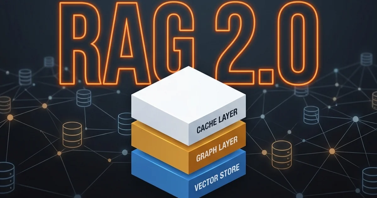
Layered Memory Tiers in RAG 2.0
Level 4 RAG systems organize enterprise memory into distinct tiers, matching how human memory stores and retrieves information.
+-----------------------------------------------------------------------+
|                       RAG 2.0 LAYERED MEMORY STACK                    |
+-----------------------------------------------------------------------+
|  Tier 1: Transient Cache Layer     | Redis / Semantic Cache           |
|  Tier 2: Structural Graph Layer    | Neo4j / Entity Relation Graph    |
|  Tier 3: Semantic Vector Layer     | pgvector / Dense Embeddings      |
|  Tier 4: System Metadata Registry  | Postgres / Relational Schemas    |
+-----------------------------------------------------------------------+- Transient Cache Layer: This layer stores frequent query patterns and their compiled context assemblies. By caching semantic equivalents using vector similarity thresholds (e.g., matching "how do I reset my credentials?" with "reset user password instructions"), the system bypasses the retrieval pipeline for common questions, reducing overall latency.
- Structural Graph Layer: This layer maps the entities (users, codebases, projects, documents) and relationships within the organization. The graph structure allows agents to perform multi-hop reasoning, helping them answer questions that trace connections across different teams and projects.
- Semantic Vector Layer: This layer stores dense vector representations of text passages. It handles conceptual searches where the user is looking for ideas rather than specific keyword matches.
- System Metadata Registry: This layer contains the core database schemas, document catalog records, access control lists (ACLs), and source files. It ensures that the retrieval system respects user permissions and accesses the most up-to-date versions of documents.
For more details on managing on-device agent storage, see our guide on Kotlin Multiplatform Compose on-device agents.
Hybrid Retrieval Mechanics: Merging BM25 Lexical Search with Dense Embeddings
To build a reliable retrieval pipeline, we must combine two different search approaches: lexical (keyword-based) search and dense vector (semantic) search.
Dense vectors excel at matching general concepts. If a user searches for "troubleshoot network delays," a vector search can successfully retrieve documents containing "diagnosing packet loss" or "latency issues," even if the specific words do not match.
However, vector search struggles when queries include exact matches like part numbers, function names, or specific serial keys (e.g., searching for sys_init_v2). In these cases, lexical algorithms like BM25 are much more reliable because they match exact characters.
+-----------------------------------------------------------------------+
|                    HYBRID RETRIEVAL PIPELINE                          |
+-----------------------------------------------------------------------+
|                           User Query                                  |
|                                |                                      |
|                +---------------+---------------+                      |
|                |                               |                      |
|         [Lexical Path]                  [Semantic Path]               |
|         BM25 Algorithm                   Dense Vectors                |
|                |                               |                      |
|                +---------------+---------------+                      |
|                                |                                      |
|                     Reciprocal Rank Fusion                            |
|                                |                                      |
|                      Cross-Encoder Reranker                           |
|                                |                                      |
|                         Target Context                                |
+-----------------------------------------------------------------------+
The Math of Reciprocal Rank Fusion (RRF)
To combine the results of keyword and vector searches, we need a normalization method that does not rely on comparing raw scores directly. BM25 scores are unbounded, whereas cosine similarity scores are restricted between -1 and 1.
Reciprocal Rank Fusion (RRF) addresses this by evaluating the relative position (rank) of a document in each search result, rather than its raw score.
The RRF score for a document $d \in D$ is calculated using the following formula:
$$RRF\Score(d \in D) = \sum{m \in M} \frac{1}{k + r_m(d)}$$
Where:
- $M$ is the set of retrieval methods (in this case, BM25 and dense vector search).
- $r_m(d)$ is the rank of document $d$ in the results of retrieval method $m$ (1-indexed).
- $k$ is a constant weighting factor that prevents low-ranked documents from disproportionately skewing the score. The standard industry value for $k$ is $60$.
- BM25 Search: Ranked $2$nd.
- Dense Vector Search: Ranked $5$th.
$$RRF\_Score(A) = \frac{1}{60 + 2} + \frac{1}{60 + 5} = \frac{1}{62} + \frac{1}{65} \approx 0.01613 + 0.01538 = 0.03151$$
By calculating this score for all returned documents, the system sorts and identifies the most relevant passages from both retrieval paths.
Reranking Pipelines: Cross-Encoder vs. Bi-Encoder
While RRF provides a solid initial ranking, it only evaluates the position of documents in search lists. To optimize the context we send to the LLM, we need to evaluate the semantic relevance of each passage more precisely. This is where rerankers come in.
Most retrieval systems use a two-stage process:
- First-Stage Retrieval (Bi-Encoder): The system uses a Bi-Encoder model to generate vector embeddings for the query and documents independently. It performs a fast vector similarity search to narrow down millions of documents to a small candidate pool (e.g., top 100).
- Second-Stage Retrieval (Cross-Encoder): The system feeds the query and each candidate document together into a Cross-Encoder model. The Cross-Encoder processes both texts simultaneously, allowing it to evaluate detailed interactions between the query and the document text.
Bi-Encoder:
Query ----> [Embedding Model] ---\
                                  +--> [Similarity Search (Fast)] -> Top Candidates
Document -> [Embedding Model] ---/

Cross-Encoder:
(Query + Candidate Document) ----> [Cross-Encoder Model] ---------> Exact Relevance Score
Although Cross-Encoders are too computationally expensive to run against millions of documents, they are highly effective for reranking the top 50 to 100 candidate documents. The reranked list ensures that only the most relevant context is sent to the LLM.
Database Implementation in PostgreSQL
You can implement a hybrid search pipeline directly in PostgreSQL using pgvector for vector similarity and standard full-text search for lexical matching.
Here is a typical schema and search query:
-- Create extension for vector storage
CREATE EXTENSION IF NOT EXISTS vector;

-- Table definition for document chunks
CREATE TABLE document_chunks (
    id SERIAL PRIMARY KEY,
    document_id INT,
    content TEXT,
    tsv_content TSVECTOR, -- For BM25 lexical search
    embedding VECTOR(1536) -- For dense vector search (e.g., OpenAI text-embedding-3-small)
);

-- Index for lexical search
CREATE INDEX idx_chunks_tsv ON document_chunks USING GIN(tsv_content);

-- Index for vector search (HNSW index for fast similarity lookup)
CREATE INDEX idx_chunks_vector ON document_chunks USING hnsw (embedding vector_cosine_ops);

-- Trigger to update tsvector on content changes
CREATE OR REPLACE FUNCTION chunks_tsv_trigger() RETURNS trigger AS $$
begin
  new.tsv_content := to_tsvector('english', new.content);
  return new;
end
$$ LANGUAGE plpgsql;

CREATE TRIGGER trg_chunks_tsv_update BEFORE INSERT OR UPDATE
    ON document_chunks FOR EACH ROW EXECUTE FUNCTION chunks_tsv_trigger();
To run a hybrid query using PostgreSQL, you can retrieve the top lexical and vector matches, combine them using RRF logic, and return the combined results:
WITH vector_search AS (
    SELECT id, ROW_NUMBER() OVER (ORDER BY embedding <=> :query_embedding) as rank
    FROM document_chunks
    ORDER BY embedding <=> :query_embedding
    LIMIT 50
),
lexical_search AS (
    SELECT id, ROW_NUMBER() OVER (ORDER BY ts_rank_cd(tsv_content, to_tsquery('english', :lexical_query)) DESC) as rank
    FROM document_chunks
    WHERE tsv_content @@ to_tsquery('english', :lexical_query)
    ORDER BY ts_rank_cd(tsv_content, to_tsquery('english', :lexical_query)) DESC
    LIMIT 50
)
SELECT
    COALESCE(v.id, l.id) AS chunk_id,
    COALESCE(1.0 / (60 + v.rank), 0.0) + COALESCE(1.0 / (60 + l.rank), 0.0) AS rrf_score
FROM vector_search v
FULL OUTER JOIN lexical_search l ON v.id = l.id
ORDER BY rrf_score DESC
LIMIT 10;
This SQL query performs both semantic and keyword searches in parallel, normalizes the ranks using RRF, and returns the top 10 most relevant chunks.
For more details on scaling database architectures, see our analysis on pgvector scaling in 2026.
Graph Memory Architectures: Entity Extraction, Relational Schemas, and Temporal Edges
While vector similarity is useful for retrieving isolated facts, it struggles with queries that span multiple documents or require understanding structural relationships. To solve this, RAG 2.0 integrates Graph Memory (GraphRAG) into the retrieval pipeline.
A GraphRAG architecture extracts key entities (such as people, projects, technologies, and locations) and their relationships from raw documents, storing them as nodes and edges in a graph database.
       [User Profile]
             |
      (contributes_to) -- [Timestamp: 2026-05-12]
             |
             v
      [Project Alpha]
             |
        (references)
             |
             v
        [pgvector]
Entity-Relation Extraction Pipelines
Constructing a graph memory database requires a parsing pipeline to extract entities and relationships from incoming text files.
+-------------------------------------------------------------------------------+
|                        GRAPH EXTRACTION PIPELINE                              |
+-------------------------------------------------------------------------------+
|  Raw Document Ingest ---> Text Segmenting ---> Entity Extraction (LLM/NLP)   |
|                                                     |                         |
|  Graph Assembly <--- Edge Verification <--- Relationship Identification       |
+-------------------------------------------------------------------------------+- Text Segmenting: Raw documents are split into logical sections (such as paragraphs or subchapters) rather than arbitrary character lengths, preserving semantic units.
- Entity Extraction: An LLM or specialized named-entity recognition (NER) model processes the text to identify key entities and classify them into predefined types (e.g.,
Developer,Repository,API). - Relationship Identification: The model scans the text to identify connections between entities, writing them as predicates (e.g.,
EXPORTS,DEPENDS_ON,DEPRECATED). - Edge Verification: The system runs validation checks to merge duplicate nodes and resolve ambiguous names (e.g., ensuring "V. Shah" and "Vatsal Shah" map to the same node).
- Graph Assembly: The verified nodes and edges are written to a graph database (such as Neo4j or an RDF store) and linked back to their source document chunks in the vector database.
The Role of Temporal Edges
In production environments, corporate data is constantly changing. Codebases are refactored, project owners change, and documents are updated. A static knowledge graph quickly becomes outdated.
Graph Memory handles this by adding temporal edges to the graph. Every edge in the database is written with metadata attributes tracking its validity window:
{
  "source": "User_Vatsal",
  "predicate": "LEAD_ARCHITECT_OF",
  "target": "Project_Alpha",
  "properties": {
    "created_at": "2026-01-10T09:00:00Z",
    "updated_at": "2026-06-18T18:30:00Z",
    "status": "active"
  }
}
If Vatsal Shah leaves Project Alpha to lead Project Beta, the relationship is not deleted. Instead, the status of the edge is set to inactive and an ended_at timestamp is added. A new active edge is then created for Project Beta.
This temporal tracking allows the agent to answer complex chronological questions, such as "who was leading Project Alpha when the database migration occurred in March?" by filtering edges based on active timestamp windows.
Designing a Unified Graph Schema
To ensure consistency across the graph database, developers must define a clear schema for nodes and edges.
Nodes:
  - Developer  { id, name, team, role }
  - Project    { id, name, repository_url, status }
  - Component  { id, name, technology_stack, version }
  - Document   { id, title, file_path, last_modified }

Edges:
  - CONTRIBUTES_TO { role, commits_count, active_since }
  - DEPENDS_ON     { type, version_constraint }
  - WRITTEN_ABOUT  { relevance_score, last_reviewed }
  - UPDATED_BY     { timestamp, commit_hash }
By indexing data using this schema, the retrieval system can combine vector search and graph traversals.
For instance, when a user asks about component dependencies, the system first uses vector search to identify the relevant Component node, and then runs a graph query to find all related projects linked by DEPENDS_ON edges.
For an in-depth analysis of graph-based retrieval architectures, see our article on GraphRAG in production.
The Agent Context Budget: Context Window Assembly and Allocation Strategy
The release of models with large context windows (ranging from 128k to over 1 million tokens) has led to a common misconception: that developers no longer need to worry about selective retrieval. Some choose to send entire documents or databases directly to the model.
In practice, this approach introduces significant challenges:
- Lost-in-the-Middle Phenomenon: Retrieval research shows that LLMs are highly effective at finding information at the very beginning or end of a prompt, but their recall accuracy drops significantly for facts located in the middle of long contexts.
- Latency and Cost: Processing 200,000 tokens for every query increases inference latency and costs. For real-time applications like IDE extensions or chat interfaces, this overhead is unacceptable.
- Attention Clogging: Dumping irrelevant text into the context window distracts the model's attention, increasing the likelihood of hallucinations or incorrect reasoning.

Partitioning the 128k Context Window
For a standard 128k token context window, the context assembly engine should allocate space dynamically based on the following budget guidelines:
+-------------------------------------------------------------------------------+
|                       CONTEXT WINDOW BUDGET ALLOCATION                        |
+-------------------------------------------------------------------------------+
|  System Guidelines & Core Instructions      | 15% (approx. 20,000 tokens)     |
|  Active Context & Graph Relations           | 25% (approx. 32,000 tokens)     |
|  Retrieved Vector Search Chunks             | 40% (approx. 51,000 tokens)     |
|  Conversation History & Chat Buffer         | 10% (approx. 13,000 tokens)     |
|  Available Slack Space (Response Buffer)    | 10% (approx. 12,000 tokens)     |
+-------------------------------------------------------------------------------+- System Guidelines & Core Instructions (15%): This segment holds the agent's persona instructions, formatting rules, active tool definitions, and system guidelines. It remains static across the session.
- Active Context & Graph Relations (25%): This section contains structural metadata, active project definitions, and entity-relation triples retrieved from the Graph Memory layer. It provides the high-level structural context of the user's environment.
- Retrieved Vector Search Chunks (40%): This is the largest segment, reserved for high-relevance text passages retrieved via the hybrid search pipeline and verified by the Cross-Encoder reranker.
- Conversation History & Chat Buffer (10%): Rather than passing the entire chat history, this block stores a sliding window of recent messages, combined with a summarized history of earlier interactions.
- Available Slack Space (10%): This space is kept empty to ensure the model has enough token capacity to generate its response without hitting context limits.
The Context Assembly Engine
The context assembly engine runs a dynamic compiler that assembles these segments before sending the prompt to the model.
+-------------------------------------------------------------------------------+
|                        CONTEXT ASSEMBLY WORKFLOW                              |
+-------------------------------------------------------------------------------+
|  Query Ingest ---> Vector & Graph Retrieval ---> Deduplication & Reranking    |
|                                                     |                         |
|  Final Prompt Assembly <--- Format Validation <--- Token Budget Fitting       |
+-------------------------------------------------------------------------------+- Query Ingest: The user's query is received and analyzed for semantic intent.
- Vector and Graph Retrieval: The system queries the database layers in parallel to fetch candidate text chunks and entity-relation paths.
- Deduplication and Reranking: The candidates are deduplicated based on source IDs, and the Cross-Encoder reranker scores their relevance relative to the query.
- Token Budget Fitting: The assembly engine reads the candidate list in order of relevance, estimating token counts using the model's tokenizer (e.g., Tiktoken). It adds candidates to the prompt template until the allocated budget limit is reached, discarding lower-relevance chunks.
- Format Validation: The compiled prompt is validated to ensure XML tags or JSON boundaries are formatted correctly.
- Final Prompt Assembly: The formatted prompt is sent to the LLM API.
For details on optimizing model sizes for local environments, see our overview of small language models (SLMs).
Naive RAG vs. RAG 2.0 vs. Fine-Tuning: An Architectural Comparison
Choosing the right data architecture requires comparing the capabilities, costs, and maintenance trade-offs of different approaches.
The following table provides a comparison of Naive RAG (v1), RAG 2.0 (Layered Memory), and Model Fine-Tuning:
| Dimension | Naive RAG (v1) | RAG 2.0 (Layered Memory) | Model Fine-Tuning |
|---|---|---|---|
| Retrieval Accuracy | Low to Medium (50% - 60% on complex benchmarks) | High (80% - 90% via hybrid & graph alignment) | Low (Fine-tuning updates style, not factual retrieval) |
| Context Window Efficiency | Low (Prone to lost-in-the-middle issues) | High (Selective context allocation budget) | Not Applicable (No external context added) |
| Multi-Hop Reasoning | Fails (Cannot connect disjointed text chunks) | Succeeds (Traverses explicit graph memory paths) | Poor (Cannot reliably link dynamic variables) |
| Access Control (ACLs) | Hard to enforce (Requires metadata hacks) | Native (Enforced at relational database query tier) | Impossible (Factual data is baked into weights) |
| Implementation Cost | Very Low (Minimal database infrastructure) | Medium (Requires hybrid databases & parsing pipelines) | Very High (GPU clusters & specialized training pipelines) |
| Knowledge Update Speed | Real-Time (Instant vector database insertions) | Real-Time (Instant graph and vector insertions) | Slow (Requires scheduled retraining jobs) |
The 2027–2030 Transition Roadmap: Hardening Enterprise Knowledge Retrieval
As enterprise agent adoption increases, organizations must plan their transition from current RAG implementations to future cognitive memory systems.
+-------------------------------------------------------------------------------+
|                            ROADMAP: 2027 - 2030                               |
+-------------------------------------------------------------------------------+
|  Phase 1 (2027): Standardization  | Establish MCP connectors, hybrid databases |
|  Phase 2 (2028): Graph-Vector   | Move to multi-modal vector-graph stores     |
|  Phase 3 (2030): Agentic Memory  | Dynamic context compilers, temporal decay  |
+-------------------------------------------------------------------------------+
Phase 1: Standardization and Protocol Alignment (2027)
The focus for 2027 is standardization. Organizations will replace proprietary database APIs with standardized integration layers based on the Model Context Protocol (MCP).
By standardizing database connections and tool schemas, developers can build modular retrieval pipelines that are independent of specific database vendors. Vector databases will also offer native BM25 search out of the box, simplifying hybrid query pipelines.
Phase 2: Graph-Vector Database Convergence (2028)
This convergence will allow developers to run queries that combine semantic vector matches and graph traversals in a single step (e.g., executing "find similar components and return their dependencies" using a single SQL or Cypher query). This change will simplify database architectures and reduce query latency.
Phase 3: Dynamic Context Compilers and Agent Memory Tiers (2030)
Agent memory will also feature automatic temporal decay, archive scheduling, and semantic grouping, functioning as an integrated cognitive operating system for the enterprise.
Actionable Implementation Playbook: What to Do Monday Morning
To transition your system from RAG 1.0 to a reliable RAG 2.0 architecture, you can begin with three concrete steps:
Step 1: Add a BM25 Sidecar to Your Vector Database
Do not rely solely on vector embeddings. Set up a BM25 search index alongside your vector database to handle keyword-based queries.
Here is a Python example using rank_bm25 to perform hybrid search and combine results using RRF ranking:
import numpy as np
from rank_bm25 import BM25Okapi

class HybridSearchEngine:
    def __init__(self, corpus_chunks):
        self.chunks = corpus_chunks
        # Tokenize corpus for BM25
        tokenized_corpus = [doc.lower().split(" ") for doc in corpus_chunks]
        self.bm25 = BM25Okapi(tokenized_corpus)

    def lexical_search(self, query, top_n=20):
        tokenized_query = query.lower().split(" ")
        scores = self.bm25.get_scores(tokenized_query)
        top_indices = np.argsort(scores)[::-1][:top_n]
        return [(self.chunks[i], i, scores[i]) for i in top_indices]

    def vector_search(self, query_embedding, database_embeddings, top_n=20):
        # Cosine similarity calculation
        dots = np.dot(database_embeddings, query_embedding)
        norms = np.linalg.norm(database_embeddings, axis=1) * np.linalg.norm(query_embedding)
        similarities = dots / norms
        top_indices = np.argsort(similarities)[::-1][:top_n]
        return [(self.chunks[i], i, similarities[i]) for i in top_indices]

    def reciprocal_rank_fusion(self, lexical_results, vector_results, k=60):
        rrf_scores = {}

        # Process lexical results
        for rank, (_, doc_idx, _) in enumerate(lexical_results, start=1):
            rrf_scores[doc_idx] = rrf_scores.get(doc_idx, 0.0) + (1.0 / (k + rank))

        # Process vector results
        for rank, (_, doc_idx, _) in enumerate(vector_results, start=1):
            rrf_scores[doc_idx] = rrf_scores.get(doc_idx, 0.0) + (1.0 / (k + rank))

        # Sort docs by RRF score
        sorted_indices = sorted(rrf_scores.keys(), key=lambda x: rrf_scores[x], reverse=True)
        return [(self.chunks[idx], idx, rrf_scores[idx]) for idx in sorted_indices]
By deploying this hybrid lookup, your retrieval pipeline will instantly become more resilient to spelling variations and product code lookups.
Step 2: Establish a Nightly Entity-Relation Extraction Job
Begin building your organization's structural memory layer by scheduling a nightly job to extract key entities and relationships from newly uploaded documents.
import json
import openai

def extract_entities_and_relationships(text_chunk):
    system_instruction = (
        "You are an expert knowledge graph compiler. "
        "Extract key technical entities (Developers, Projects, Components) "
        "and their relationships (DEPENDS_ON, CONTRIBUTES_TO, DEVELOPED_BY) "
        "from the provided text. Return the output as JSON."
    )

    response = openai.chat.completions.create(
        model="gpt-4o-mini",
        response_format={"type": "json_object"},
        messages=[
            {"role": "system", "content": system_instruction},
            {"role": "user", "content": f"Text to parse:\n\n{text_chunk}"}
        ]
    )

    return json.loads(response.choices[0].message.content)
Save these JSON payloads to a file and run an ingestion job to write them as nodes and edges in your graph database.
Step 3: Implement an Evaluation Suite Measuring Recall@5
Establish a baseline measurement for your retrieval pipeline. Create a test suite of 50 common user questions, compile their expected reference documents, and measure retrieval recall rates before and after implementing RAG 2.0 features.
def calculate_recall_at_n(evaluation_dataset, retrieval_function, n=5):
    """
    evaluation_dataset: list of dicts with keys 'query' and 'ground_truth_chunk_ids'
    retrieval_function: function taking a query and returning list of retrieved chunk_ids
    """
    total_recall = 0.0

    for item in evaluation_dataset:
        query = item['query']
        ground_truth = set(item['ground_truth_chunk_ids'])

        # Retrieve candidate chunks
        retrieved = set(retrieval_function(query, top_n=n))

        # Calculate intersection
        matches = ground_truth.intersection(retrieved)
        recall = len(matches) / len(ground_truth) if len(ground_truth) > 0 else 0.0
        total_recall += recall

    mean_recall = total_recall / len(evaluation_dataset)
    return mean_recall
By measuring this metric regularly, you can verify if changes to chunk sizes, embedding models, or reranking pipelines are improving retrieval accuracy.
References and Sources
- BM25 Search Algorithm: Robertson, S., & Zaragoza, H. (2009). The Probabilistic Relevance Framework: BM25 and Beyond. Foundations and Trends in Information Retrieval, 3(4), 333-380.
- Reciprocal Rank Fusion: Cormack, G. V., Clarke, C. L. A., & Buettcher, S. (2009). Reciprocal Rank Fusion Outperforms Landoff and Condorcet. ACM SIGIR Conference on Research and Development in Information Retrieval, 580-587.
- Cross-Encoder Reranking: Nogueira, R., & Cho, K. (2019). Passage Re-ranking with BERT. arXiv preprint arXiv:1901.04085.
- GraphRAG Architecture: Edge, D., Trinh, H., Cheng, B., et al. (2024). From Local Retrieve-and-Read to Global Summarization: A GraphRAG Approach. arXiv preprint arXiv:2404.16130.
- Context Window Attention: Liu, N. F., Lin, K., Chen, J., et al. (2023). Lost in the Middle: How Language Models Use Long Contexts. arXiv preprint arXiv:2307.03172.